Feature Analysis for Classification (Iris)

Background

Before training a classifier you look at two things: how each feature is distributed within each class, and whether the classes are separable in feature space. This study uses the classic Iris dataset — three species, four measurements — to reproduce those two views with the convenience marks.

Class-conditional distributions

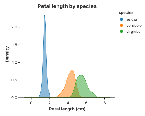
mark_density reads the feature from x and gives one curve per color group, so you can see how a feature separates the classes. Petal length is clearly bimodal: setosa sits far to the left, while versicolor and virginica overlap in the middle. A single threshold on this feature would split setosa perfectly but confuse the other two.

Feature separation

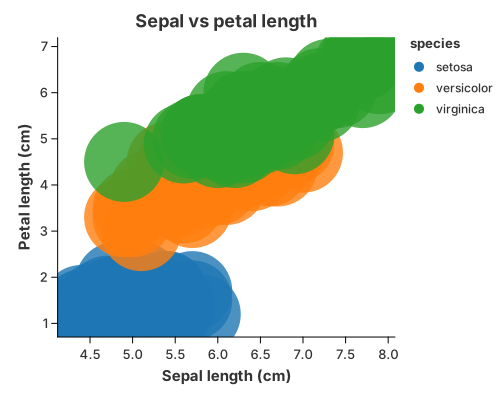
A scatter of two features, coloured by class, shows the decision boundary a linear model would try to find. Setosa is linearly separable from the other two; versicolor and virginica share a region where any straight boundary has to trade false positives for false negatives.

Implementation

//! Case study: exploratory feature analysis before training a classifier.
//!
//! Two views you would actually look at on the Iris dataset:
//!
//! 1. the **class-conditional distribution** of a feature (is it separable?),
//! 2. a **scatter of two features**, coloured by class, to see the decision
//!    boundary a linear model would find.

use charton::prelude::*;
use std::error::Error;

fn main() -> Result<(), Box<dyn Error>> {
    let iris = load_dataset("iris")?;

    // 1. Class-conditional density of petal length.
    chart!(&iris)?
        .mark_density()?
        .configure_density(|density| density.with_opacity(0.5))
        .encode((alt::x("petal_length"), alt::color("species")))?
        .with_title("Petal length by species")
        .with_x_label("Petal length (cm)")
        .with_y_label("Density")
        .save("docs/src/images/case_data_science_density.svg")?;

    // 2. Two features, coloured by class. Setosa is linearly separable from the
    //    other two; versicolor and virginica overlap.
    chart!(&iris)?
        .mark_point()?
        .configure_point(|point| point.with_size(40.0).with_opacity(0.8))
        .encode((
            alt::x("sepal_length"),
            alt::y("petal_length"),
            alt::color("species"),
        ))?
        .with_title("Sepal vs petal length")
        .with_x_label("Sepal length (cm)")
        .with_y_label("Petal length (cm)")
        .save("docs/src/images/case_data_science_scatter.svg")?;

    println!("Saved case_data_science_density.svg and case_data_science_scatter.svg");
    Ok(())
}

Both figures are a single encoding each: y/x for the values and color for the class. The axis and legend titles come from the original columns (petal_length, sepal_length, species) automatically.

What it demonstrates

• mark_density for class-conditional distributions, one curve per group.
• mark_point + color for feature separation and decision boundaries.
• The grammar behind both: a density is transform_density + mark_area; a scatter is mark_point. See 1-D Density and Scatter.

See also

• Violin — the same distributions as an outline with an inner box.
• 2-D Density — the joint distribution of two features.
• Scatter matrices — the full pairwise view.