Contour Plots

A contour plot draws the lines (or bands) where a scalar field equals a set of levels.

mark_contour is the convenient way to draw one. It is a composite mark: behind the scenes it expands into the ordinary recipe

contour = iso-line stat (marching squares)  +  open-path geometry

so the general pieces stay available. transform_contour works on any regular grid of x, y and z — an elevation map, a pressure field, a bivariate density — and mark_path draws any ordered polyline.

Iso-lines of a grid

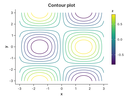
Name the scalar field explicitly (the crate has no z channel) and read x/y from the encodings. The lines are coloured by their level by default.

//! Contour plot — the convenience `mark_contour`.
//!
//! `mark_contour` is a **composite** mark: it expands into the public
//! `transform_contour` (marching squares over a regular grid) and the shared
//! open-path renderer. For the composition written out by hand, see
//! `contour_manual.rs`.
//!
//! The scalar field `z` is named explicitly because the crate has no `z`
//! channel; `x` and `y` come from the encodings. By default the lines are
//! coloured by their level.

use charton::prelude::*;
use std::error::Error;

fn main() -> Result<(), Box<dyn Error>> {
    // Sample z = sin(x) * cos(y) on a regular grid.
    let n = 41;
    let mut x = Vec::new();
    let mut y = Vec::new();
    let mut z = Vec::new();
    for i in 0..n {
        for j in 0..n {
            let xv = -3.0 + 6.0 * i as f64 / (n as f64 - 1.0);
            let yv = -3.0 + 6.0 * j as f64 / (n as f64 - 1.0);
            x.push(xv);
            y.push(yv);
            z.push((xv).sin() * (yv).cos());
        }
    }

    chart!(x, y, z)?
        .mark_contour("z")?
        .configure_contour(|contour| contour.with_levels(10).with_stroke_width(1.5))
        .encode((alt::x("x"), alt::y("y")))?
        .configure_theme(|t| t.with_color_map(ColorMap::Viridis))
        .with_title("Contour plot")
        .with_x_label("x")
        .with_y_label("y")
        .save("docs/src/images/contour.svg")?;

    println!("Saved docs/src/images/contour.svg");
    Ok(())
}

What the transforms produce

Both steps replace the table, so to wire them together by hand you need to know the columns each one emits. The full contract is in the transforms reference; for a contour the two names that matter are:

path_group is not built in: it is an ordinary data column, and mark_path connects the rows that share it, in row order. You wire it to the path_group channel with alt::path_group("path_group").
level is each line's value. Map it to color to colour the lines, or drop the colour encoding for a single-colour contour. mark_contour does this colour mapping for you by default.

Every emitted name is only a default output name. Rename it with ContourTransform::with_as and ContourTransform::with_level_as, then use the new names downstream — see the transforms reference.

How the pieces fit

Piece	What it does	Reused by
`transform_contour`	marching squares over a regular grid → iso-lines	contours of any scalar field, density contours
`transform_density_2d`	bivariate kernel density over a grid	density contours, density heatmaps
`mark_contour`	the `transform_contour` + open-path composite	ready-made contour plots
`mark_path`	connects a `path_group` in row order, open, stroked	contour lines, custom curves, parallel coordinates
`mark_polygon`	the closed, filled form of the same geometry	violin outlines, maps, filled ribbons

Why mark_path and not mark_polygon? A contour is a line: some contours are open (they end on the plot edge), others are loops, but in both cases we want the stroke, not a filled disc. mark_polygon would close every open contour with a spurious edge and fill every loop. See Connecting the dots.

ContourTransform accepts either a number of evenly spaced levels (with_levels(n)) or explicit ones (with_levels_values(vec![...])); configure_contour exposes those as with_levels(n) / with_levels_values(...).

Colouring the lines by level is optional. Turn it off with configure_contour(…).with_color_by_level(false) and the path is drawn with the mark's own stroke instead — a single-colour contour:

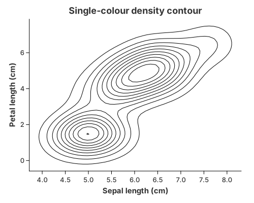
//! Single-colour density contour, with `mark_contour`.
//!
//! The same iso-lines as `density_contour.rs`, but with the marks'
//! colour-by-level turned off, so every line uses the outline colour instead.

use charton::prelude::*;
use std::error::Error;

fn main() -> Result<(), Box<dyn Error>> {
    let iris = load_dataset("iris")?;

    chart!(&iris)?
        .transform_density_2d(
            // Pad the estimation grid so the outer iso-lines close before its
            // edge instead of being clipped by it.
            Density2DTransform::new("sepal_length", "petal_length")
                .with_grid_size(60)
                .with_padding(0.3),
        )?
        .mark_contour("density")?
        .configure_contour(|contour| {
            contour
                .with_levels(10)
                .with_color_by_level(false)
                .with_stroke("black")
                .with_stroke_width(1.0)
        })
        .encode((alt::x("x"), alt::y("y")))?
        .with_title("Single-colour density contour")
        .with_x_label("Sepal length (cm)")
        .with_y_label("Petal length (cm)")
        .save("docs/src/images/contour_single.svg")?;

    println!("Saved docs/src/images/contour_single.svg");
    Ok(())
}

From scattered points

A bivariate density is just another scalar grid, so transform_density_2d feeds mark_contour("density") — the familiar kdeplot / geom_density_2d picture. The grid can also be drawn filled instead of as lines. Both are on the 2-D Density page:

scatter  →  transform_density_2d  →  mark_contour

Built from the primitives

The same picture without mark_contour: transform_contour turns the grid into polylines and mark_path draws them, coloured by level.

//! Contour plot — built by hand from the primitives.
//!
//! The same picture as `contour.rs`, without `mark_contour`. A contour is a
//! **composition**, not a dedicated chart type:
//!
//! ```text
//! contour = iso-line stat (marching squares)  +  open-path geometry
//! ```
//!
//! * `transform_contour` (marching squares) turns a gridded `z` into
//!   `(x, y, path_group, level)` polylines;
//! * `mark_path` draws those polylines, coloured by `level`.
//!
//! The scalar grid is *your* data, so `transform_contour` reads `x`, `y`, `z`
//! and replaces the table with `x`, `y`, `path_group`, `level`. In `encode` you
//! then map those columns to channels: `x`/`y` to the axes, `path_group` groups
//! the vertices into separate lines, and `level` colours each line.

use charton::prelude::*;
use std::error::Error;

fn main() -> Result<(), Box<dyn Error>> {
    // Sample z = sin(x) * cos(y) on a regular grid.
    let n = 41;
    let mut x = Vec::new();
    let mut y = Vec::new();
    let mut z = Vec::new();
    for i in 0..n {
        for j in 0..n {
            let xv = -3.0 + 6.0 * i as f64 / (n as f64 - 1.0);
            let yv = -3.0 + 6.0 * j as f64 / (n as f64 - 1.0);
            x.push(xv);
            y.push(yv);
            z.push((xv).sin() * (yv).cos());
        }
    }

    chart!(x, y, z)?
        .transform_contour(ContourTransform::new("x", "y", "z").with_levels(10))?
        .mark_path()?
        .configure_path(|m| m.with_stroke_width(1.5))
        .encode((
            alt::x("x"),
            alt::y("y"),
            alt::path_group("path_group"),
            alt::color("level"),
        ))?
        .configure_theme(|t| t.with_color_map(ColorMap::Viridis))
        .with_title("Contour plot")
        .with_x_label("x")
        .with_y_label("y")
        .save("target/example-output/contour_manual.svg")?;

    println!("Saved target/example-output/contour_manual.svg");
    Ok(())
}

Charton: The Grammar of Graphics in Rust