Heatmaps
A heatmap is mark_rect over two position axes, coloured by a value. The only
question is whether the axes are categorical or continuous.
Categorical heatmap
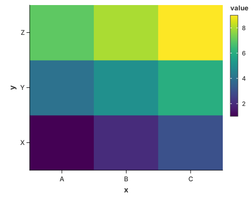
Each (x, y) pair is one cell, coloured by its value.
//! Heatmap over two **categorical** axes.
//!
//! Each `(x, y)` pair is one cell, coloured by its value. Continuous axes use
//! the same mark with automatic binning — see `heatmap_rect.rs`.

use charton::prelude::*;
use std::error::Error;

fn main() -> Result<(), Box<dyn Error>> {
    // Sample data for heatmap
    let x = ["A", "B", "C", "A", "B", "C", "A", "B", "C"];
    let y = ["X", "X", "X", "Y", "Y", "Y", "Z", "Z", "Z"];
    let value = [1.0, 2.0, 3.0, 4.0, 5.0, 6.0, 7.0, 8.0, 9.0];

    // Create heatmap chart
    chart!(x, y, value)?
        .mark_rect()?
        .encode((alt::x("x"), alt::y("y"), alt::color("value")))?
        .save("docs/src/images/heatmap.svg")?;

    Ok(())
}
Continuous heatmap (2-D binning)
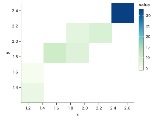
The same mark with automatic binning on both axes — a "2-D histogram" heatmap.
//! Heatmap over two **continuous** columns.
//!
//! `mark_rect` slices the x and y axes into a grid and paints each cell with the
//! colour of the value that falls in it. This is the "2D density heatmap" shape;
//! for the iso-lines of a density instead, see `density_contour.rs`.

use charton::prelude::*;
use std::error::Error;

fn main() -> Result<(), Box<dyn Error>> {
    // Sample data for heatmap with continuous variables
    let x = [1.1, 1.2, 1.3, 1.4, 1.5, 1.6, 1.8, 2.05, 2.2, 2.5, 2.6, 2.7];
    let y = [1.2, 1.3, 1.4, 1.5, 1.8, 1.83, 2.0, 1.9, 2.2, 2.3, 2.4, 2.5];
    let value = [
        1.0, 2.0, 3.0, 4.0, 5.0, 6.0, 7.0, 8.0, 9.0, 10.0, 11.0, 12.0,
    ];
    // Create heatmap chart
    chart!(x, y, value)?
        .mark_rect()?
        .encode((alt::x("x"), alt::y("y"), alt::color("value")))?
        .configure_theme(|t| t.with_color_map(ColorMap::GnBu))
        .save("docs/src/images/heatmap_rect.svg")?;

    Ok(())
}
See also
- Contour Plots — the smooth, iso-line alternative to a binned heatmap, including density contours.