Composing Your Own

The convenience marks cover the charts people ask for by name. This page is for everything else: how to assemble the public transforms and the Tier-1 geometries into a picture that no mark provides.

Read Design Rules: Marks, Tiers & Statistical Atoms for the tiers and the thin-recipe rule, and Transforms & Columns for the column each transform emits.

The pattern

A hand-written recipe is always three steps:

1. stat — a transform_* replaces the table with derived columns;
2. geom — a Tier-1 mark draws those columns;
3. encode — map the emitted columns to channels (x, y, path_group, color).

Every convenience mark is exactly this, and its expansion is written out on its own page under "Built from the primitives":

A new composition: the mirrored density

Recombining means choosing a different geom for the same stat — or the other way round. mark_violin pairs transform_density with transform_band (a mirrored polygon). Pair the same density with mark_area and stack: "center" instead and you get a mirrored density: each curve is drawn from -density / 2 to +density / 2. This is the Vega-Lite density + area + stack recipe, and it is the right choice when you want the untrimmed tail rather than the data-bounded violin.

//! Mirrored density — a new picture recombined from the primitives.
//!
//! `mark_violin` pairs `transform_density` with `transform_band` (a mirrored
//! polygon). This example pairs the *same* statistic with `mark_area` and
//! `stack: "center"` instead: each curve is drawn from `-density / 2` to
//! `+density / 2`, then `coord_flip` stands it upright. It is the Vega-Lite
//! `density + area + stack` recipe, and it keeps the untrimmed tail rather than
//! stopping at the data like a violin.

use charton::prelude::*;
use std::error::Error;

fn main() -> Result<(), Box<dyn Error>> {
    let iris = load_dataset("iris")?;

    chart!(iris)?
        .transform_density(
            DensityTransform::new("sepal_length")
                .with_as("sepal_length", "density")
                .with_groupbys(["species"]),
        )?
        .mark_area()?
        .configure_area(|area| area.with_opacity(0.6).with_stroke("#2c3e50"))
        .encode((
            alt::x("sepal_length"),
            alt::y("density").with_stack("center"),
            alt::color("species"),
        ))?
        .coord_flip()
        .with_title("Mirrored density")
        .with_x_label("Density")
        .with_y_label("Sepal length (cm)")
        .save("target/example-output/density_mirror.svg")?;

    println!("Saved target/example-output/density_mirror.svg");
    Ok(())
}

A ridgeline from a half-band

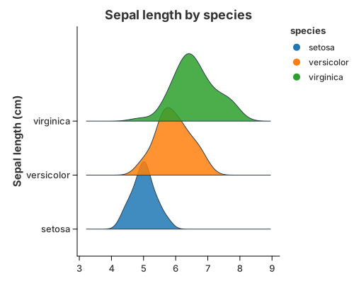
A ridgeline stacks one density per category, each sitting on its baseline and overlapping the one above. mark_violin uses a symmetric band; transform_band(…).with_side(BandSide::Right) keeps only one bank, so the flat edge of the polygon is the baseline. with_overlap(2.5) grows each ridge past its lane so the densities overlap, and coord_flip puts the value on the horizontal axis and the density bulge on the vertical one.

//! Ridgeline — one density per category, each sitting on its baseline.
//!
//! This is a composition, not a mark. The density comes from
//! `transform_density`; `transform_band(…).with_side(BandSide::Right)` turns each
//! curve into a one-sided band whose flat edge is the category baseline; and
//! `coord_flip` puts the value on the horizontal axis and the density bulge on
//! the vertical one. `with_overlap` lets each ridge grow past its lane so it
//! overlaps the one above it. A ridge is a violin that keeps one bank.
//!
//! The category axis is trained from the numeric positions the band emits, so
//! the tallest ridge is never clipped even though it grows past the last
//! category. The recipe needs no hand-written expansion.

use charton::prelude::*;
use std::error::Error;

fn main() -> Result<(), Box<dyn Error>> {
    let iris = load_dataset("iris")?;

    chart!(iris)?
        .transform_density(
            DensityTransform::new("sepal_length")
                .with_as("sepal_length", "density")
                .with_groupbys(["species"]),
        )?
        .transform_band(
            BandTransform::new("sepal_length", "density")
                .with_center("species")
                .with_side(BandSide::Right)
                .with_width(1.0)
                .with_overlap(2.5)
                .with_scale(BandScale::PerGroup),
        )?
        .mark_polygon()?
        .configure_geoshape(|mark| {
            mark.with_opacity(0.85)
                .with_stroke("#2c3e50")
                .with_stroke_width(1.0)
        })
        .encode((
            // The category axis covers the band's real extent automatically:
            // a ridge grows past its lane, and the scale expands to include it.
            alt::x("x").with_category_labels("species"),
            alt::y("y"),
            alt::path_group("path_group"),
            alt::color("species"),
        ))?
        .coord_flip()
        .with_title("Sepal length by species")
        .with_x_label("Sepal length (cm)")
        .with_y_label("")
        .save("docs/src/images/ridge.svg")?;

    println!("Saved docs/src/images/ridge.svg");
    Ok(())
}

The pieces are all public: transform_density estimates one curve per category, transform_band mirrors it into a polygon and mark_polygon fills it. None of this is ridge-specific: with_side(BandSide::Both) is the full violin, a one-sided band is a half violin, and with_overlap is also how violins overlap. See The firewall for why a ridgeline is a recipe rather than a mark.

One practical note: because a ridge grows past its lane, the category axis is trained from the numeric positions the band actually emits. The axis expands to include them, so the example needs no hand-written with_expansion; use it only when you want more (or less) breathing room than the automatic fit.

Choosing the geometry

For anything that "connects the dots", the geometry differs by exactly two flags: open or closed and sorted by x or in row order.

So a contour (mark_path, open) and a violin (mark_polygon, closed) are the same geometry one flag apart. See Connecting the dots.

When to stop composing

If you keep rebuilding the same picture, that is the signal to add a mark — but only if it passes the promotion checklist. A split violin is a parameter of mark_violin; a raincloud is a stack of layers, so it stays a recipe. The rule of thumb: a name that is a geometry/statistic atom (violin, contour) can become a mark; a name that is a metaphor for a whole picture (raincloud, waterfall) is a composition.

See also

• Transforms & Columns — the full column contract.
• Marks & Geometries — the Tier-1 vocabulary (mark_point, mark_path, mark_polygon, …).
• Design Rules — tiers, the thin-recipe rule, and when a new mark is justified.