2-D Density

A two-dimensional density estimate describes the joint distribution of two numeric columns. transform_density_2d estimates it on a regular grid; the same grid can then be drawn two ways, both as composite marks:

transform_density_2d                 // (x, y)  →  (x, y, density) grid
  ├─ mark_density_2d                 // filled density heatmap
  └─ mark_contour("density")         // iso-density lines

Neither mark hides anything: they expand into transform_density_2d plus the public mark_rect / transform_contour geometry, so the hand-written recipe is always available (see the column contract).

Density heatmap

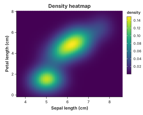
Read the two columns from x and y; the mark estimates the joint density and paints one cell per grid node, coloured by the density.

//! Density heatmap — a bivariate kernel density drawn as a grid of cells, with
//! `mark_density_2d`.
//!
//! `mark_density_2d` is a **composite** mark: it expands into the public
//! `transform_density_2d` and the shared rectangle geometry. It sets the heatmap
//! bin count to the grid size automatically, so the caller does not have to know
//! that `mark_rect` bins a second time. This is the filled counterpart of the
//! density contour.

use charton::prelude::*;
use std::error::Error;

fn main() -> Result<(), Box<dyn Error>> {
    let iris = load_dataset("iris")?;

    chart!(iris)?
        .mark_density_2d()?
        .configure_density_2d(|density| density.with_grid_size(60).with_padding(0.2))
        .encode((alt::x("sepal_length"), alt::y("petal_length")))?
        .configure_theme(|t| t.with_color_map(ColorMap::Viridis))
        .with_title("Density heatmap")
        .with_x_label("Sepal length (cm)")
        .with_y_label("Petal length (cm)")
        .save("docs/src/images/density_heatmap.svg")?;

    println!("Saved docs/src/images/density_heatmap.svg");
    Ok(())
}

Building it by hand is transform_density_2d followed by mark_rect. mark_rect paints one cell per grid node, so you must set the x and y bins to the grid size or the cells get merged back together — mark_density_2d does that for you.

Density contours

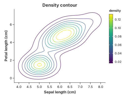
The same grid can be passed to mark_contour("density"), which turns it into iso-lines. Colour them by level for the familiar kdeplot / geom_density_2d picture, or drop the colour for a single-colour contour.

//! Density contour — iso-lines of a bivariate kernel density, with
//! `mark_contour`.
//!
//! The scattered points are first summarised into a density grid by the public
//! `transform_density_2d`, then `mark_contour("density")` turns that grid into
//! iso-lines and draws them. So the mark handles the contouring; the density
//! estimate stays an explicit, reusable step.

use charton::prelude::*;
use std::error::Error;

fn main() -> Result<(), Box<dyn Error>> {
    let iris = load_dataset("iris")?;

    chart!(iris)?
        // 1. Estimate the joint density of the two measurements.
        .transform_density_2d(
            // Pad the estimation grid so the outer iso-lines close before its
            // edge instead of being clipped by it.
            Density2DTransform::new("sepal_length", "petal_length")
                .with_grid_size(60)
                .with_padding(0.3),
        )?
        // 2. Extract and draw iso-density lines (coloured by level by default).
        .mark_contour("density")?
        .configure_contour(|contour| contour.with_levels(8).with_stroke_width(1.2))
        .encode((alt::x("x"), alt::y("y")))?
        .configure_theme(|t| t.with_color_map(ColorMap::Viridis))
        .with_title("Density contour")
        .with_x_label("Sepal length (cm)")
        .with_y_label("Petal length (cm)")
        .save("docs/src/images/density_contour.svg")?;

    println!("Saved docs/src/images/density_contour.svg");
    Ok(())
}

The column contract

When you build these by hand, both steps replace the table, so you need to know the columns each one emits:

density is consumed by the contour step, so it never appears in encode. Rename the outputs with Density2DTransform::with_as and ContourTransform::with_as / with_level_as. This is the canonical list for both transforms; the hand-written wire-up is on the Contour Plots page.

Tuning the estimate

configure_density_2d forwards the estimator options:

For a contour, a dashed line is configure_contour(\|m\| m.with_dash([6.0, 4.0])).

See also

• Contour Plots — the general marching-squares contour, for any scalar grid.
• Heatmaps — mark_rect over binned data.
• Composing Your Own — recombining the primitives into new pictures.
• Transforms & Columns.